How the PolyBlocks AI Compiler Works#
Authored by: PolyMage team
July 2024
Note: For a detailed writeup on PolyBlocks, please see this arXiv paper instead.
Introduction#
Compilers are back#
Compilers are one of the major areas that comprise the systems discipline of Computer Science, with Operating Systems, Networks, Databases, and Programming Languages being some of the other major disciplines. While languages like C, C++, Java, and Rust come to mind first when people think of compilers as a traditional area, ‘Compilers for AI’ or building compilers that accelerate Python-based AI programming frameworks is one of the most promising and challenging areas in modern systems research and development.
Python-based AI programming frameworks like PyTorch, JAX, and TensorFlow are pretty popular, with one framework overtaking or catching up with another at various times. While Python is interpreted and known to be extremely slow compared to compiled languages, these frameworks do not suffer from that issue largely – if they did, all of the astounding progress that AI has made using high-performance computing (HPC) would not have been possible. These frameworks are typically fast because they rely on highly optimized and tuned libraries that were written in CUDA, C, C++, or machine assembly. As such, the heavy lifting is done by calls to those libraries instead of the “glue” code in Python.
Downsides of libraries#
Library-based execution suffers from “locally” optimized execution, i.e., the operators run fast, but performance is lost or limited at the boundaries of those operators’ execution. Transfers to global memory are performed, and performance is quickly memory bandwidth bound and nowhere close to the arithmetic intensity that is achievable. A common pitfall here is to conclude that the computation is bandwidth-bound and nothing could be done other than increasing the hardware memory bandwidth. This is a common pre-mature conclusion that precludes attempts at further optimization. Fusion across operators allows one to perform more computation for the same memory bandwidth, the importance of which is well-established. This has led to one of the following two strategies for mitigation:
hand-written libraries for well-known fused operators like matmul-bias-add-relu or attention (flash-attention)
“semi-compiler” approaches, i.e., systems that map to libraries as well as perform compilation where it’s feasible. Torch Inductor (torch.compile) from the official PyTorch repository, NVIDIA TensorRT, and XLA are some semi-compiler systems that make use of libraries and elements of compilation to varying extents depending on the input.
We call the systems in (2) “semi-compilers” since they heavily rely on hand-written libraries as well for performance. In most cases, this is by design to enable good performance while layering on top of existing hand-optimization already done, while in other cases, for pragmatic reasons, awaiting further improvements to the compiler.
Advances in computer architecture#
While the late 90s and early 2000s saw multiple cores on a chip and then more and more cores as well as wider SIMD up to an extent, the late 2000s saw “many-core” architectures (“GPUs”), which later turned into a revolution. Specialized units to perform matrix multiplication (“tensor cores”) arrived on GPUs in the 2010s. Interestingly, similar architectures (in the form of systolic arrays) were the usual subject of architecture research up until the early 90s; they were killed by the advent of superscalar microprocessors (“PC” revolution) in the early 90s, and later commodity clusters of such systems. These systems became easy to compile for and use. More interestingly, we are now back with such systolic-like arrays or other designs as specialized units on more general-purpose many-core processors to accelerate certain computations in the AI domain (matmuls, convolutions, and constructs built on top of those).
Besides increasing core count (more SMs on GPUs), providing higher bandwidth to these cores and more tensor cores, a trend in the last five years has been the ability to exploit lower precision for the AI domain of computations, perfectly matched with hardware support for such lower or mixed precision from 16-bit to 8 or 4-bit, both floating-point and fixed-point (integer).
We will see that a part of this article is on effectively exploiting such lower-precision units and requires good compiler support.
Building modern compilers and MLIR#
Building compilers for Python-based AI frameworks or building domain-specific compilers, in general, was always hard until 2019 because the developers of such systems had to invent or re-invent intermediate representation and other key compiler infrastructure. LLVM was the only low-level infrastructure that had been available, and it had been inadequate to build compilers for high-level frameworks. XLA and Halide are examples of two systems (for different domains) that created their own intermediate representations or operator sets and subsequently compiled those down to LLVM. All of these and other new intermediate representations were not built to serve as a general and principled IR infrastructure for high-productivity languages. This changed with the arrival of MLIR into open source in 2019.
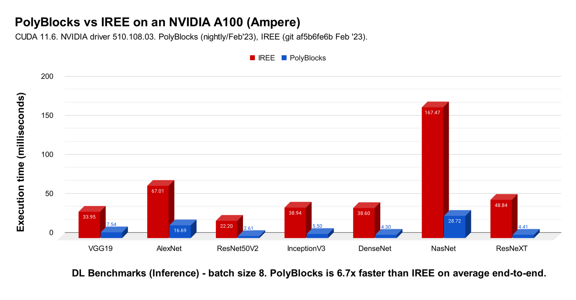
MLIR provided a toolkit to build new domain-specific compilers without having to create completely new IRs and their infrastructure. More information on MLIR concepts can be found on its official page. Unfortunately, there are no effective open-source MLIR-based AI compilers: the ones that exist have major technical limitations, being nowhere close to the level of performance, range of optimizations, stability/coverage, or framework integration of XLA or Torch Inductor. To the best of our knowledge, no MLIR-based compiler (outside of PolyBlocks) has claimed performance close to “semi-compilers” like XLA or Torch Inductor on substantial workloads nor demonstrated the one-liner incremental integration with AI programming frameworks.
While MLIR adoption took time, other systems like TensorRT and PyTorch incorporated compilers or elements of compilation into their frameworks with their own intermediate representations. Numerous DL compiler systems (too many to name) were built or experimented with by the academic community as well, all without a proper compiler infrastructure and thus not suitable to last and evolve.
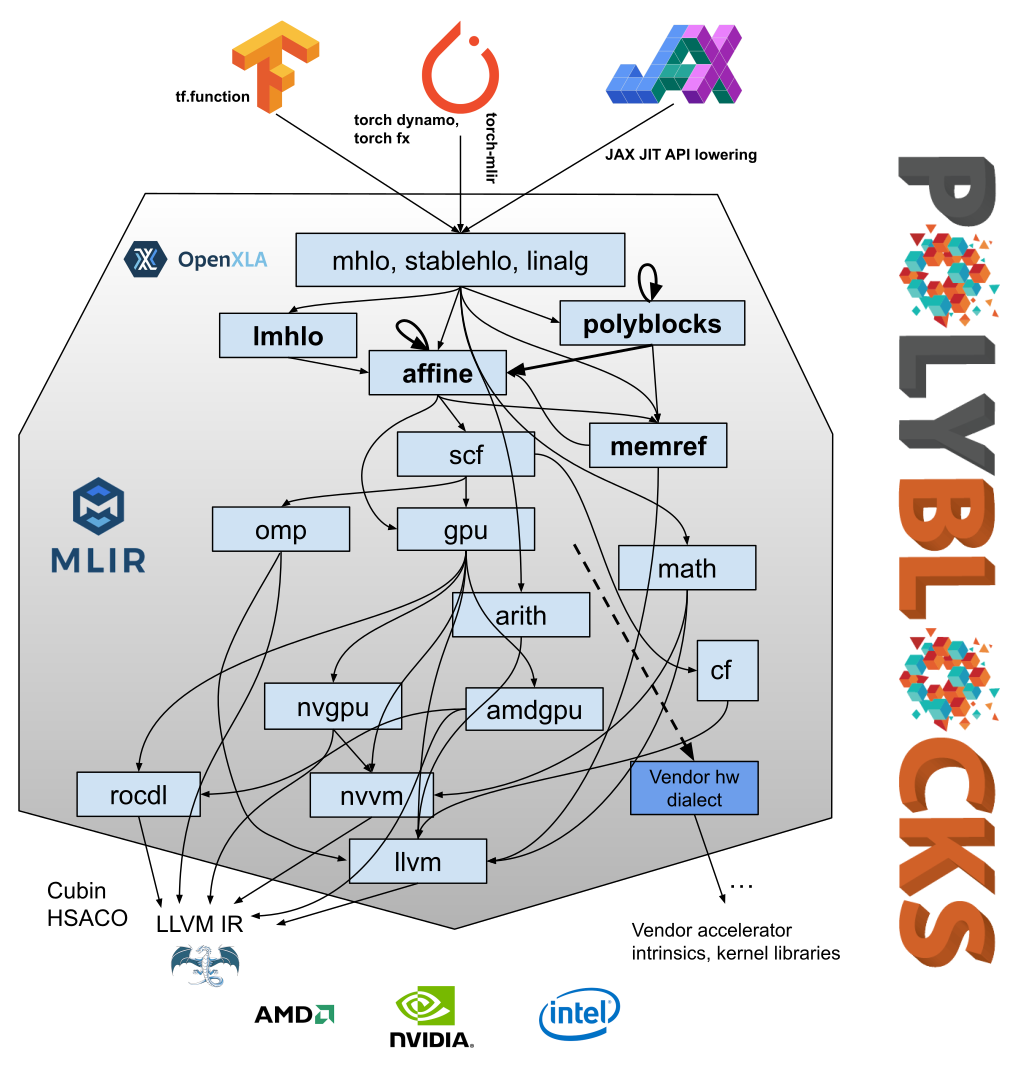
PolyBlocks#
PolyBlocks from Polymage Labs is a 100% code-generating, fully automatic, and analytical model-driven compiler engine based on MLIR. It can be viewed as an MLIR-based pass pipeline with 200+ passes that transform and optimize IR through various stages. It mainly employs polyhedral abstractions and optimization techniques in the mid-level stages while optimizing computations on high-dimensional data spaces. The optimization techniques encompass tiling, fusion, performing recomputation (in conjunction with tiling and fusion), packing into on-chip buffers for improved locality, eliminating intermediate tensors or shrinking intermediate tensors to bounded buffers fitting into on-chip memory, mapping to matmul/tensor cores, and efficient parallelization in a way unified with all other transformations. Several MLIR upstream passes are also used in the PolyBlocks’ code generation pipeline. Unlike XLA, TensorRT, or Torch Inductor, PolyBlocks does not rely on any hand-written code, kernels, or libraries to pattern match to and substitute, i.e., no libraries like CUTLASS, CUDNN, CUBLAS, ROC-BLAS, flash attention, or any cu* kernels or their variants are used.
In the context of domain-specific compilers or ML/AI compilers, the term “code-generating” is used to distinguish from “pattern-match” and map to pre-written code. “Traditional” compilers like GCC and Clang (LLVM-based) generate all their code (there may be rare exceptions to this though, where low-level libraries may be used to substitute incoming IR).
Usability#
From a usability standpoint, PolyBlocks provides seamless integration with PyTorch, JAX, and TensorFlow, requiring a one-line annotation or a call to JIT compile or AOT compile. As an example, here’s how a PyTorch function is annotated to compile and execute on GPUs without the need to know anything about CUDA, and run five times as fast here than torch.compile on an NVIDIA GPU.
@polyblocks_jit_torch(compile_options={'target': 'nvgpu'})
def blur_x_blur_y(img):
  # We are doing a regular image convolution in the X direction and then in
  # the Y direction.
  kernel = torch.tensor([0.0625, 0.25, 0.375, 0.25, 0.0625],
                        device = img.device).float()
  blur_kernel = kernel.view(1, 1, 1, 5)
  img_reshaped = img.view(3, 1, height, width)
  # The output is two short at each end.
  blurx = torch.nn.functional.conv2d(img_reshaped,
                                     blur_kernel, stride=1, padding=0)
  blur_kernel = kernel.view(1, 1, 5, 1)
  blury = torch.nn.functional.conv2d(blurx, blur_kernel,
                                     stride=1, padding=0)
  output = blury.View(3, height - 4, width - 4)
  return output
Besides PolyBlocks, such a one-line incremental framework integration is also provided by XLA, Torch Inductor (torch.compiler), and a few other non-MLIR compilers.
PolyBlocks compiler transformations#
A compiler for deep learning AI computations largely deals with operations on dense tensors. The key capabilities of a good compiler for this domain include the following optimizations:
Fusing across operators.
Performing tiling for locality and parallelism.
Mapping computations to tensor/matmul cores or similar specialized units.
Ability to tile and fuse without losing the ability to parallelize, vectorize, and map to specialized units where available.
Performing redundant computation to avoid global memory accesses where profitable.
Utilize on-chip shared memory when possible.
Vectorization.
Parallelization that is adequate and dealing with excess parallelism.
Register tiling or unroll-and-jam.
Reordering execution for better spatial, temporal, and group reuse.
A long list of other traditional/”textbook” compiler optimizations like folding, sub-expression elimination, simplification, canonicalization, invariant code motion, and scalar replacement of subscripted accesses.
Deep unified pass pipeline#
The PolyBlocks compiler engine organizes the above optimizations in passes and applies them as part of a long pass pipeline comprising 200+ passes. The passes are divided into five stages, and a major part of the above optimizations happens in the third stage, which comprises a sequence of about 100+ passes. The lower stages of the pipeline largely include upstream MLIR repository passes unchanged. The same pass pipeline is used for all incoming IR, regardless of whether they are from PyTorch, TensorFlow, or JAX and regardless of what kind of AI models are being compiled. The list of passes is identical for NVIDIA and AMD GPUs, while CPUs use a shorter list, which is effectively a strict subset, with some differences for the lower part of the pipeline. The pipeline separation between targeting CPUs and CPUs + GPU-like devices is mainly for convenience to avoid running a large number of “no-op” passes when compiling for CPUs. The passes in the pipeline have a mechanism to look up target information and other metadata that may be attached by previous passes as and when needed to correctly compile and specialize transformations. All of these passes typically take from a couple of seconds to a few tens of seconds to compile large AI models.
Mapping to tensor cores#
The anatomy of a loop nest targeted to GPU tensor cores in its mid-level form is shown below. The nest below explains about a dozen concepts in the IR representation of optimized code: it shows how multi-level parallelism can be represented in MLIR (using affine.parallel ops) and mapped to the GPU parallelism hierarchy. The snippet below is not fully optimized, but it shows warp-level primitives (gpu.subgroup_mma* operations), copy-in and copy-out between global memory and on-chip scratchpads (GPU shared memory), computation on the tensor cores happening in mixed precision (f16 input and f32 output), and 128-bit vector load/stores to speed up data movement between global memory and shared memory.
// Grid of thread blocks.
affine.parallel (%arg3) = (0) to (379) {
  %alloc = memref.alloc() : memref<128x136xf16, 3>
  %alloc_5 = memref.alloc() {alignment = 16 : i64} : memref<128x16xf16, 3>
  %7 = memref.vector_cast %alloc_5 : memref<128x16xf16, 3> to memref<128x2xvector<8xf16>, 3>
  %alloc_6 = memref.alloc() : memref<128x12xf32, 3>
  affine.parallel (%arg4, %arg5) = (0, 0) to (min(128, %arg3 * -128 + 48400), 3) {
    affine.store %cst_0, %alloc_6[%arg4, %arg5] : memref<128x12xf32, 3>
  }
  // Warp-level parallelism.
  affine.parallel (%arg4) = (0) to (4) {
    %8 = affine.apply affine_map<(d0) -> (d0 * 32)>(%arg4)
    %9 = gpu.subgroup_mma_load_matrix %alloc_6[%8, %c0] {leadDimension = 12 : index} : memref<128x12xf32, 3> -> !gpu.mma_matrix<32x8xf32, "COp">
    // Threads of a thread block. Copy-in from global memory.
    affine.parallel (%arg5, %arg6) = (0, 0) to (128, 128) {
      %11 = affine.load %memref[0, ((%arg5 + %arg3 * 128) floordiv 220 + (%arg6 floordiv 3) floordiv 5) mod 224, ((%arg5 + %arg3 * 128) mod 220 + %arg6 floordiv 3 - ((%arg6 floordiv 3) floordiv 5) * 5) mod 224, %arg6 mod 3] : memref<1x224x224x3xf16>
      affine.store %11, %alloc[%arg5, %arg6] : memref<128x136xf16, 3>
    }
    // Threads of a thread block. Copy-in from global memory.
    affine.parallel (%arg5, %arg6) = (0, 0) to (128, 8) {
      %11 = affine.load %memref_1[((%arg5 floordiv 3) floordiv 5) mod 5, (%arg5 floordiv 3) mod 5, %arg5 mod 3, %arg6 mod 3] : memref<5x5x3x3xf16>
      affine.store %11, %alloc_5[%arg5, %arg6] : memref<128x16xf16, 3>
    }
    // Zero init.
    affine.parallel (%arg5) = (0) to (53) {
      affine.store %cst, %7[%arg5 + 75, 0] : memref<128x2xvector<8xf16>, 3>
    }
    %10 = affine.for %arg5 = 0 to 8 iter_args(%arg6 = %9) -> (!gpu.mma_matrix<32x8xf32, "COp">) {
      %11 = affine.apply affine_map<(d0) -> (d0 * 16)>(%arg5)
      %12 = affine.apply affine_map<(d0) -> (d0 * 32)>(%arg4)
      %13 = gpu.subgroup_mma_load_matrix %alloc[%12, %11] {leadDimension = 136 : index} : memref<128x136xf16, 3> -> !gpu.mma_matrix<32x16xf16, "AOp">
      %14 = gpu.subgroup_mma_load_matrix %alloc_5[%11, %c0] {leadDimension = 16 : index} : memref<128x16xf16, 3> -> !gpu.mma_matrix<16x8xf16, "BOp">
      // Warp-level primitives.
      %15 = gpu.subgroup_mma_compute %13, %14, %arg6 : !gpu.mma_matrix<32x16xf16, "AOp">, !gpu.mma_matrix<16x8xf16, "BOp"> -> !gpu.mma_matrix<32x8xf32, "COp">
      affine.yield %15 : !gpu.mma_matrix<32x8xf32, "COp">
    }
    gpu.subgroup_mma_store_matrix %10, %alloc_6[%8, %c0] {leadDimension = 12 : index} : !gpu.mma_matrix<32x8xf32, "COp">, memref<128x12xf32, 3>
  }
  memref.dealloc %alloc_5 : memref<128x16xf16, 3>
  memref.dealloc %alloc : memref<128x136xf16, 3>
  // Threads of a thread block. Copy-out to global memory.
  affine.parallel (%arg4, %arg5) = (0, 0) to (min(128, %arg3 * -128 + 48400), 3) {
    %8 = affine.load %alloc_6[%arg4, %arg5] : memref<128x12xf32, 3>
    %9 = arith.truncf %8 : f32 to f16
    affine.store %9, %memref_3[0, (%arg4 + %arg3 * 128) floordiv 220, (%arg4 + %arg3 * 128) mod 220, %arg5] : memref<1x220x220x3xf16>
  }
  memref.dealloc %alloc_6 : memref<128x12xf32, 3>
}
memref<128x2xvector<8xf16>, 3> is a type that represents a buffer of 2048
16-bit float values organized as a 128x2 matrix of 8-wide 16-bit float elements.
The trailing 3 indicates the memory space of this buffer, which, in this case,
maps to the GPU’s shared memory.
We observe three levels of parallelism here: grid-level, warp-level, and thread block-level. Warp-level parallelism is referred to here since the WMMA primitives used to model execution on tensor cores are warp-level or warp-cooperative: all threads in a warp work together in a synchronized manner to execute those operations as viewed by a programmer or the compiler emitting such IR.
The snippet also shows how affine functions are used to express complex but
“regular” packing of data so that matmul units can be used to execute the
convolution. The loop nests that move data between global memory (default memory
space of 0) and the shared memory before and after the actual compute nest can
be seen.
The tail of the nest also exhibits a trivial fusion: the truncation from fp32 to fp16 is fused with the kernel executing the matrix-matrix multiplication. This means fp16 data values leave the chip as opposed to 32-bit, transferring half as much data. This transformation happens within the pass pipeline during the polyhedral fusion pass.
In summary, a code generator has complete control at a desired level of abstraction, abstracting detail away from passes that precede this form, and allow subsequent passes to expand out and optimize further.
Quantization: exploiting low precision#
Resource-limited hardware like edge devices, where computational capabilities and device memory are limited, benefit from exploiting lower-precision computation for model inference. Quantization accomplishes this by converting model weights from high-precision floating point formats like FP32 to low-precision integer formats like INT8. Quantization is particularly useful during inference as it requires significantly less memory footprint, and saves a lot of computation cost with an acceptable loss of inference accuracy. Directly casting the weights stored as high-precision floating point formats to the 256 values of INT8 could lead to an accuracy loss. Instead, values are scaled based on scale and zero-point values of weight and activation tensors on a per-channel, per-layer, or per-tensor level.
PolyBlocks supports PyTorch models quantized using Quantization 2.0 workflow. All optimization that works on non-quantized models, like fusion, vectorization, tensor-core mapping, etc., works out of the box for quantized models. This is an extremely productive workflow for using quantization with an MLIR-based compiler. An example is shown below.
# Quantized PyTorch ResNet50 inference.
import copy
import torch
import torch._dynamo as torchdynamo
from resnet50_quantizer_utils import get_symmetric_quantization_config, BackendQuantizer
import torchvision
from torch.ao.quantization.quantize_pt2e import (
    convert_pt2e,
    prepare_pt2e,
)
from polyblocks.torch_polyblocks_compiler import polyblocks_jit_torch
from polyblocks.common_utils import validate_outputs
from torchvision.models impot resnet50, ResNet50_Weights

if __name__ == "__main__":
    example_inputs = (torch.randn(1, 3, 224, 224),)
    model = resnet50(weights=ResNet50_Weights.DEFAULT, progress=True).eval()
    # Program capture.
    exported_model, guards = torchdynamo.export(
        model,
        *copy.deepcopy(example_inputs),
        aten_graph=True,
    )
    quantizer = BackendQuantizer()
    operator_config = get_symmetric_quantization_config()
    quantizer.set_global(operator_config)

    # Prepare the model for PTQ.
    prepared_model = prepare_pt2e(exported_model, quantizer)
    # Calibrate/train the model.
    after_prepare_result = prepared_model(*example_inputs)
    # Convert back the calibrated/trained model to the quantized model.
    quantized_model = convert_pt2e(prepared_model, fold_quantize=True)
    print("converted module is: {}".format(quantized_model), flush=True)

    # Perform ResNet50_V2 inference via PolyBlocks.
    polyblocks_quantized_resnet50_inference = polyblocks_jit_torch(
        compile_options={'target': 'nvgpu'}
    )(quantized_model)

    image = torch.randn(1, 3, 224, 224)
    out = polyblocks_quantized_resnet50_inference(image)
We will discuss significant performance benefits with such quantization in a section further below.
The PolyBlocks compiler also supports quantization for TensorFlow with a similarly usable workflow, the details of which, with an example, can be found here.
Putting everything into action#
An example showing the fusion of nearly 15-20 operators into the output of a quantized tensor-core mapped convolution is shown in the snippet below. A basic introduction to MLIR is required for a better understanding of the IR snippet. This example shows tiling, fusion, mapping to tensor cores, and vectorization. Some literature refers to this kind of fusion as “consumer” fusion or tail fusion since it involves fusing pointwise operators at the tail of a heavier matmul computation.
        // Tensor core mapped compute on a tile.
        ...
        %520 = gpu.subgroup_mma_compute %508, %519, %arg166 {b_transpose} : !gpu.mma_matrix<16x16xi8, "AOp">, !gpu.mma_matrix<16x16xi8, "BOp"> -> !gpu.mma_matrix<16x16xi32, "COp">
        %521 = gpu.subgroup_mma_compute %511, %519, %arg167 {b_transpose} : !gpu.mma_matrix<16x16xi8, "AOp">, !gpu.mma_matrix<16x16xi8, "BOp"> -> !gpu.mma_matrix<16x16xi32, "COp">
        affine.yield %510, %512, %514, %515, %517, %518, %520, %521 : !gpu.mma_matrix<16x16xi32, "COp">, !gpu.mma_matrix<16x16xi32, "COp">, !gpu.mma_matrix<16x16xi32, "COp">, !gpu.mma_matrix<16x16xi32, "COp">, !gpu.mma_matrix<16x16xi32, "COp">, !gpu.mma_matrix<16x16xi32, "COp">, !gpu.mma_matrix<16x16xi32, "COp">, !gpu.mma_matrix<16x16xi32, "COp">
      }
      gpu.barrier
      gpu.subgroup_mma_store_matrix %506#0, %view_574[%494, %c0] {leadDimension = 68 : index} : !gpu.mma_matrix<16x16xi32, "COp">, memref<128x68xi32, 3>
      gpu.subgroup_mma_store_matrix %506#1, %view_574[%496, %c0] {leadDimension = 68 : index} : !gpu.mma_matrix<16x16xi32, "COp">, memref<128x68xi32, 3>
      gpu.subgroup_mma_store_matrix %506#2, %view_574[%494, %c16] {leadDimension = 68 : index} : !gpu.mma_matrix<16x16xi32, "COp">, memref<128x68xi32, 3>
      gpu.subgroup_mma_store_matrix %506#3, %view_574[%496, %c16] {leadDimension = 68 : index} : !gpu.mma_matrix<16x16xi32, "COp">, memref<128x68xi32, 3>
      gpu.subgroup_mma_store_matrix %506#4, %view_574[%494, %c32] {leadDimension = 68 : index} : !gpu.mma_matrix<16x16xi32, "COp">, memref<128x68xi32, 3>
      gpu.subgroup_mma_store_matrix %506#5, %view_574[%496, %c32] {leadDimension = 68 : index} : !gpu.mma_matrix<16x16xi32, "COp">, memref<128x68xi32, 3>
      gpu.subgroup_mma_store_matrix %506#6, %view_574[%494, %c48] {leadDimension = 68 : index} : !gpu.mma_matrix<16x16xi32, "COp">, memref<128x68xi32, 3>
      gpu.subgroup_mma_store_matrix %506#7, %view_574[%496, %c48] {leadDimension = 68 : index} : !gpu.mma_matrix<16x16xi32, "COp">, memref<128x68xi32, 3>
    }
    affine.parallel (%arg158, %arg159) = (0, 0) to (128, 16) {
      %494 = affine.load %493[%arg158, %arg159] : memref<128x17xvector<4xi32>, 3>
      %495 = arith.sitofp %494 : vector<4xi32> to vector<4xf32>
      %496 = affine.load %10[%arg159] : memref<16xvector<4xf32>>
      %497 = arith.mulf %495, %496 : vector<4xf32>
      %498 = affine.load %11[%arg159] : memref<16xvector<4xf32>>
      %499 = arith.addf %497, %498 : vector<4xf32>
      %500 = arith.divf %499, %cst_35 : vector<4xf32>
      %501 = math.roundeven %500 : vector<4xf32>
      %502 = arith.maximumf %501, %cst_6 : vector<4xf32>
      %503 = arith.minimumf %502, %cst_5 : vector<4xf32>
      %504 = arith.fptosi %503 : vector<4xf32> to vector<4xi8>
      %505 = arith.sitofp %504 : vector<4xi8> to vector<4xf32>
      %506 = affine.load %12[%arg159] : memref<16xvector<4xf32>>
      %507 = arith.truncf %cst_61 : f64 to f32
      %508 = vector.splat %507 : vector<4xf32>
      %509 = arith.addf %506, %508 : vector<4xf32>
      %510 = vector.extract %509[0] : vector<4xf32>
      %511 = math.sqrt %510 : f32
      %512 = vector.insert %511, %509 [0] : f32 into vector<4xf32>
      %513 = vector.extract %509[1] : vector<4xf32>
      %514 = math.sqrt %513 : f32
      %515 = vector.insert %514, %512 [1] : f32 into vector<4xf32>
      %516 = vector.extract %509[2] : vector<4xf32>
      %517 = math.sqrt %516 : f32 loc(#loc526
      %518 = vector.insert %517, %515 [2] : f32 into vector<4xf32>
      %519 = vector.extract %509[3] : vector<4xf32>
      %520 = math.sqrt %519 : f32
      %521 = vector.insert %520, %518 [3] : f32 into vector<4xf32>
      %522 = arith.mulf %505, %cst_35 : vector<4xf32>
      %523 = arith.divf %cst_2, %521 : vector<4xf32>
      %524 = affine.load %13[%arg159] : memref<16xvector<4xf32>>
      %525 = arith.subf %522, %524 : vector<4xf32>
      %526 = arith.mulf %525, %523 : vector<4xf32>
      %527 = affine.load %14[%arg159] : memref<16xvector<4xf32>>
      %528 = arith.mulf %526, %527 : vector<4xf32>
      %529 = affine.load %15[%arg159] : memref<16xvector<4xf32>>
      %530 = arith.addf %528, %529 : vector<4xf32>
      %531 = arith.cmpf ugt, %530, %cst_0 : vector<4xf32>
      %532 = arith.select %531, %530, %cst_0 : vector<4xi1>, vector<4xf32>
      %533 = arith.divf %532, %cst_34 : vector<4xf32>
      %534 = math.roundeven %533 : vector<4xf32>
      %535 = arith.maximumf %534, %cst_6 : vector<4xf32>
      %536 = arith.minimumf %535, %cst_5 : vector<4xf32>
      %537 = arith.fptosi %536 : vector<4xf32> to vector<4xi8>
      affine.store %537, %17[%arg157 floordiv 800, ((%arg158 + %arg157 * 128) mod 102400) floordiv 320, (%arg158 + %arg157 * 128) mod 320, %arg159] : memref<8x320x320x16xvector<4xi8>>
  }
}
A snippet from the PTX assembly generated from the MLIR above is shown below indicating the use of int-based tensor core matmul instructions.
      ...
      wmma.load.b.sync.aligned.col.m16n16k16.shared.s8        {%r1798, %r1799}, [%rd52], %r898;
      wmma.mma.sync.aligned.row.col.m16n16k16.s32.s8.s8.s32
              {%r1800, %r1801, %r1802, %r1803, %r1804, %r1805, %r1806, %r1807},
              {%r1740, %r1741},
              {%r1798, %r1799},
              {%r1724, %r1725, %r1726, %r1727, %r1728, %r1729, %r1730, %r1731};
      ...
Performance#
The results below are on an NVIDIA A10, a tensor-core equipped data-center-class GPU based on the NVIDIA Ampere architecture. The A10 is often considered to provide a good cost/performance tradeoff for inference compared to the A100.
Batch sizes one and eight exercise different workload characteristics. The former is essential for real-time vision inference scenarios, while the latter for offline use or more “bulk” processing and with more parallelism to better utilize the hardware parallelism available.
How does this compare with a similarly usable approach?#

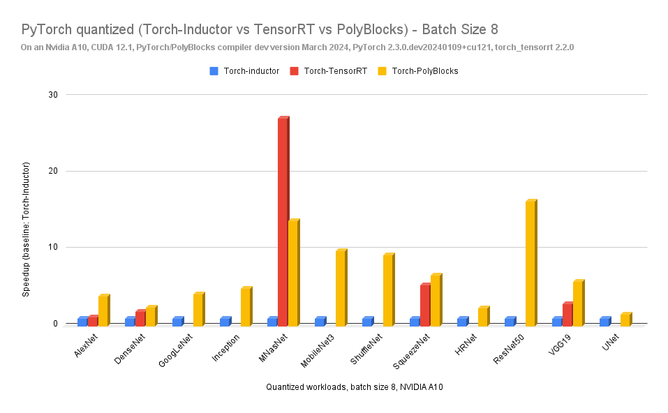
The results above show dramatic speedups over TorchInductor when quantizing. We believe this is also partly because there is limited optimization and support for such quantized models, and the torch compiler has more work to do here. TensorRT crashed/failed while handling the quantization of many of these models.
We are comparing approaches that have a similar level of usability, and hence the comparison with TorchInductor. TensorRT is another framework that can be used to quantize PyTorch models, but its usability is nowhere close to the approach described above, and it does not provide the fine-grained control that PyTorch Quantization 2.0 does.
How much does quantization help?#
The chart below shows how much improvement we readily get by quantizing, switching from fp16 to i8 simply by adding the few lines described in the previous section.
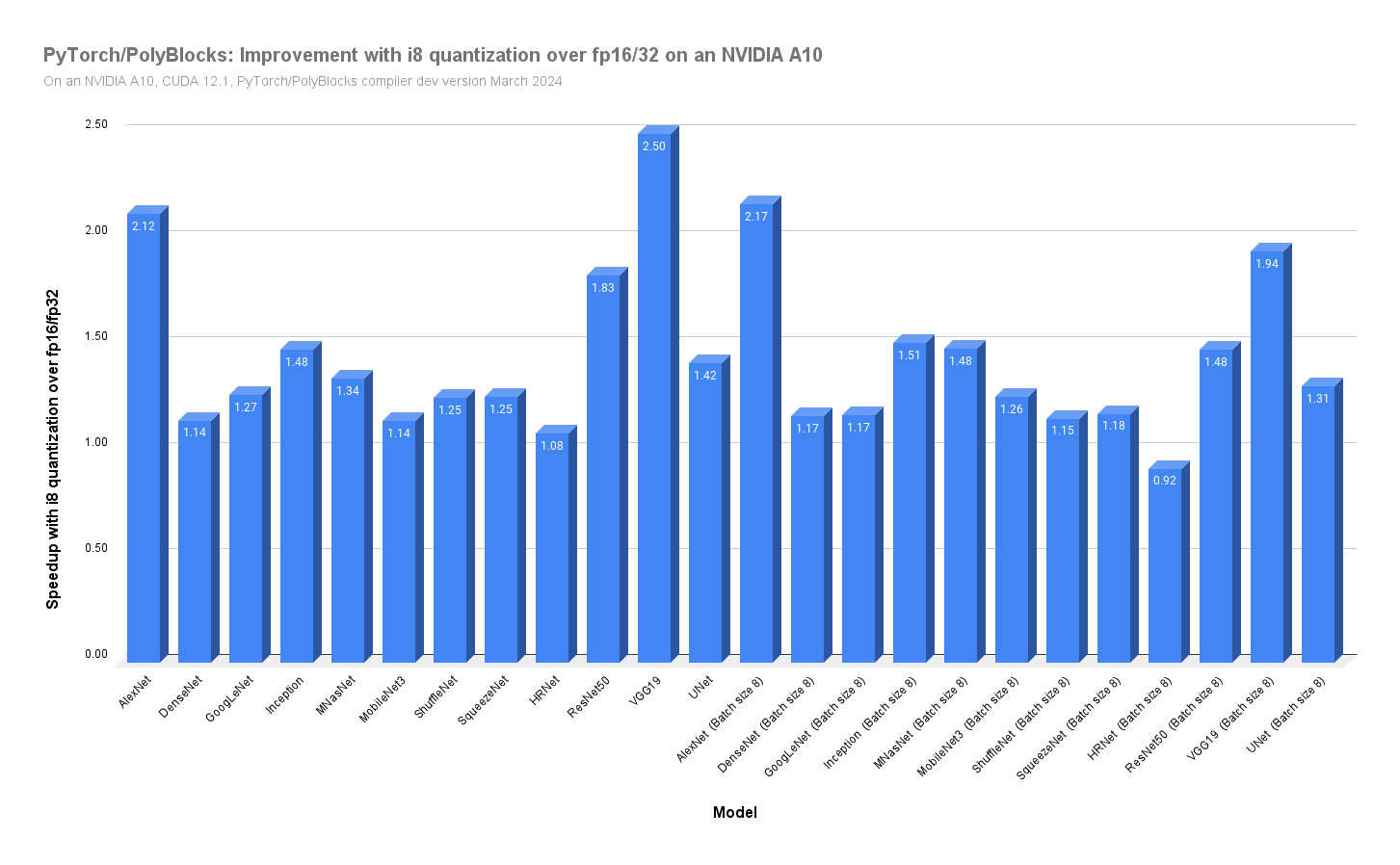
Ideally, we would expect two times as fast performance with int8 over fp16 (minus quantization overheads). Question to the readers: what could be the reasons for more than a 2x improvement in some cases? While we think about that, we see on average an improvement of about 1.5x over a number of large vision models.
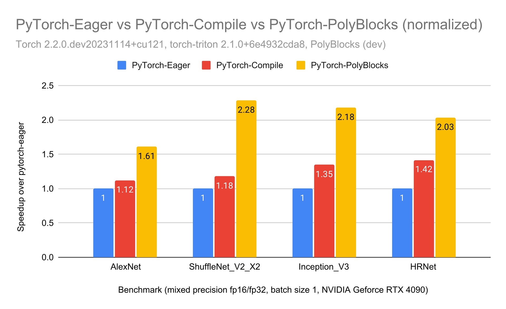
Improvements with mixed precision#
While PolyBlocks is still a work in progress with more optimizations to be implemented in the coming weeks, its performance has already reached a point where it is three times as fast as PyTorch standard (non-compiled) and even about 2x as fast as Torch Inductor (the current production-strength compiler for PyTorch) on some workloads.
PolyBlocks-generated code yields faster and fewer (more/better fused and tiled) GPU kernels and involves less overhead. It also doesn’t use CUTLASS, CUBLAS, flash attention, or any cu* kernels or their variants. Everything is generated via compiler passes on MLIR.
The input in all these cases are Python PyTorch functions and the compiler-generated code does not use anything pre-written/pre-compiled in C, C++, CUDA, or assembly, outside of standard runtime calls for memory allocation/deallocation, data transfer, and synchronization. The PolyBlocks compiler itself is written in C++, having been built using MLIR and LLVM.
Some results on vision workloads based on convolutional neural networks.
PolyBlocks also supports cross-reduction operator fusion, but this will be the subject of a future article. Such an optimization significantly improves the performance of the attention layer used in transformer-based models. A sneak preview of those results on certain attention layer configurations and on a few transformer-based models from HuggingFace are shown below.
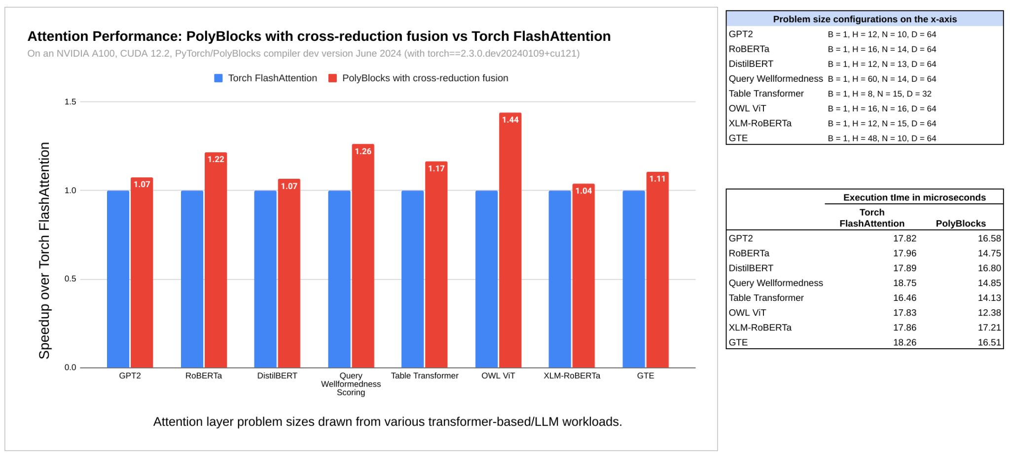
![]()
What’s next?#
There are several optimizations that the PolyBlocks compiler engine does not yet perform, and these will further improve the performance of the code it generates. So, improvements over existing approaches are expected to widen. Stay tuned for more by following us on LinkedIn and Twitter.
References and additional information#
PyTorch 2 paper at ASPLOS 2024 – a recent publication for an excellent and comprehensive introduction to end-to-end compilation for AI programming frameworks.